Lesson 5

 

Introduction

A function is a predefined formula that performs calculations using specific values in a particular order. All spreadsheet programs include common functions that can be used for quickly finding the sum, average, count, maximum value, and minimum value for a range of cells. In order to use functions correctly, you'll need to understand the different parts of a function and how to create arguments to calculate values and cell references.

The parts of a function

In order to work correctly, a function must be written a specific way, which is called the syntax. The basic syntax for a function is an equals sign (=), the function name (SUM, for example), and one or more arguments. Arguments contain the information you want to calculate. The function in the example below would add the values of the cell range A1:A20.

Working with arguments

Arguments can refer to both individual cells and cell ranges and must be enclosed within parentheses. You can include one argument or multiple arguments, depending on the syntax required for the function.

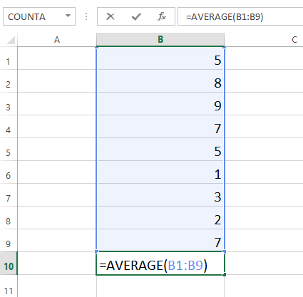
For example, the function =AVERAGE(B1:B9) would calculate the average of the values in the cell range B1:B9. This function contains only one argument.

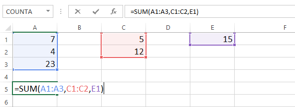
Multiple arguments must be separated by a comma. For example, the function =SUM(A1:A3, C1:C2, E2) will add the values of all cells in the three arguments.

Let's practice!

Question 1 of 1

Which of the following functions is using the correct syntax?

=A2:A8(SUM)E2:E8

SUM(A2:A8,E2:E8)=

=SUM(A2:A8,E2:E8)

SUM=(A2:A8,E2:E8)

Using functions

There are a variety of functions. Here are some of the most common functions you'll use:

• SUM: This function adds all the values of the cells in the argument.
• AVERAGE: This function determines the average of the values included in the argument. It calculates the sum of the cells and then divides that value by the number of cells in the argument.
• COUNT: This function counts the number of cells with numerical data in the argument. This function is useful for quickly counting items in a cell range.
• MAX: This function determines the highest cell value included in the argument.
• MIN: This function determines the lowest cell value included in the argument.

To use a function:

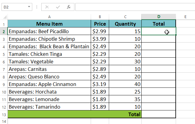
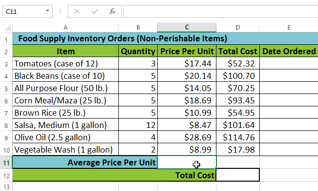
In our example below, we'll use a basic function to calculate the average price per unit for a list of recently ordered items using the AVERAGE function.

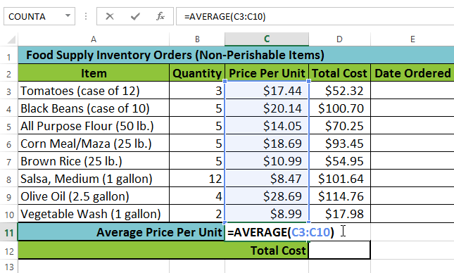
1. Select the cell that will contain the function. In our example, we'll select cell C11.
   
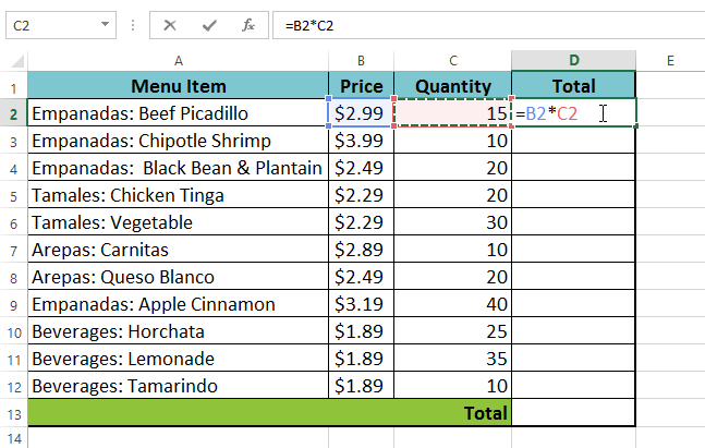
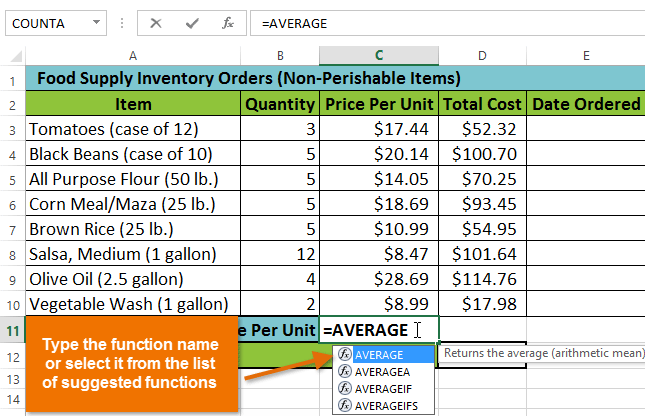
2. Type the equals sign (=) and enter the desired function name. In our example, we'll type =AVERAGE.
   
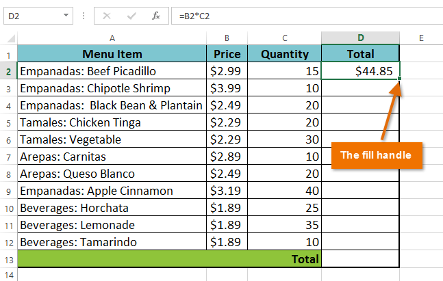
3. Enter the cell range for the argument inside parentheses. In our example, we'll type (C3:C10). This formula will add the values of cells C3:C10 and then divide that value by the total number of cells in the range to determine the average.
   
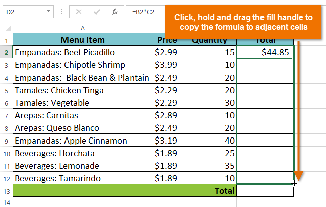
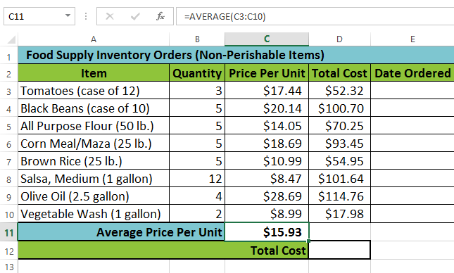
4. Press Enter on your keyboard. The function will be calculated, and the result will appear in the cell. In our example, the average price per unit of items ordered was $15.93.
   

Your spreadsheet will not always tell you if your function contains an error, so it's up to you to check all of your functions. To learn how to do this, check out the Double-Check Your Formulas lesson.

Let's practice!

Question 1 of 1

In this example, we want to use the formula =MAX(B3:D7)

What would that formula find?

The smallest amount of an item ordered in March

The total number of items sold between January and March

The largest amount of an item ordered between January and March

The average number of cakes sold in March

Working with unfamiliar functions

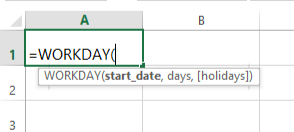
If you want to learn how a function works, you can start typing that function in a blank cell to see what it does.

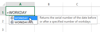
You can then type an open parenthesis to see what kind of arguments it needs.

Understanding nested functions

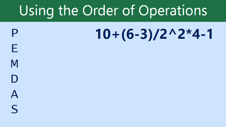
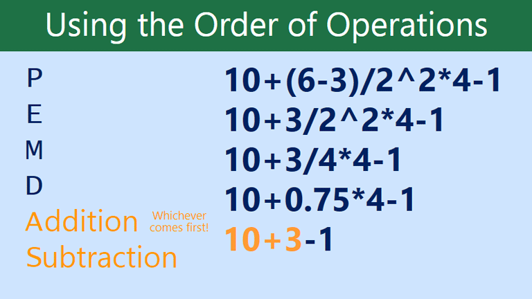
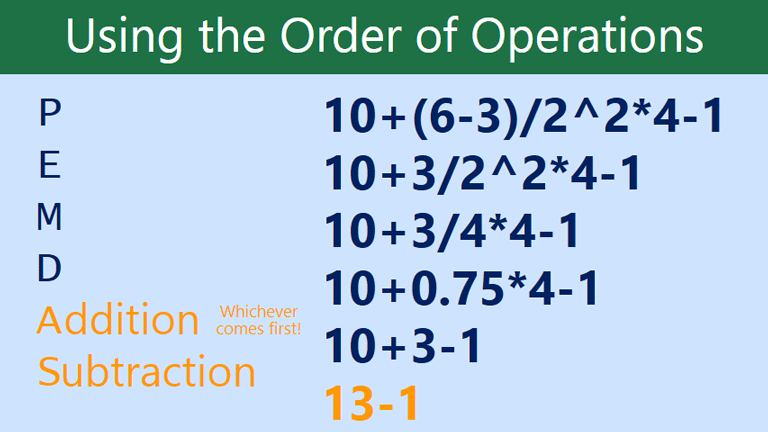
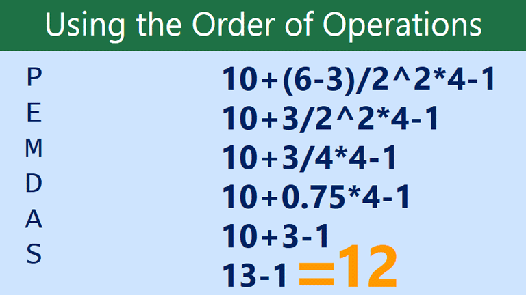
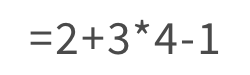
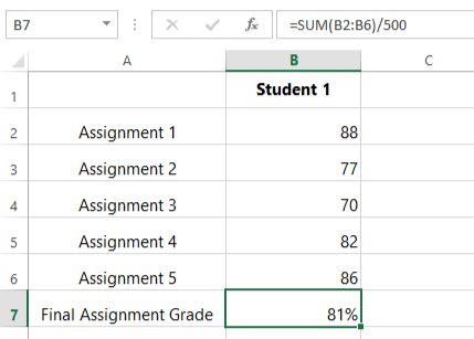
Whenever a formula contains a function, the function is generally calculated before any other operators, like multiplication and division. That's because the formula treats the entire function as a single value—before it can use that value in the formula, it needs to run the function. For example, in the formula below, the SUM function will be calculated before division:

Let's take a look at a more complicated example that uses multiple functions:

=WORKDAY(TODAY(),3)

Here, we have two different functions working together: the WORKDAY function and the TODAY function. These are known as nested functions, since one function is placed, or nested, within the arguments of another. As a rule, the nested function is always calculated first, just like parentheses are performed first in the order of operations. In this example, the TODAY function will be calculated first, since it's nested within the WORKDAY function.

Lesson 4

 Lesson 4: Relative and Absolute Cell References

Introduction

There are two types of cell references: relative and absolute. Relative and absolute references behave differently when copied and filled to other cells. Relative references change when a formula is copied to another cell. Absolute references, on the other hand, remain constant no matter where they are copied.

Relative references

By default, all cell references are relative references. When copied across multiple cells, they change based on the relative position of rows and columns. For example, if you copy the formula =A1+B1 from row 1 to row 2, the formula will become =A2+B2. Relative references are especially convenient whenever you need to repeat the same calculation across multiple rows or columns.

To create and copy a formula using relative references:

In the following example, we want to create a formula that will multiply each item's price by the quantity. Rather than create a new formula for each row, we can create a single formula in cell D2 and then copy it to the other rows. We'll use relative references so the formula correctly calculates the total for each item.

1. Select the cell that will contain the formula. In our example, we'll select cell D2.
   
2. Enter the formula to calculate the desired value. In our example, we'll type =B2*C2.
   
3. Press Enter on your keyboard. The formula will be calculated, and the result will be displayed in the cell.
4. Locate the fill handle in the lower-right corner of the desired cell. In our example, we'll locate the fill handle for cell D2.
   
5. Click, hold, and drag the fill handle over the cells you wish to fill. In our example, we'll select cells D3:D12.
   
6. Release the mouse. The formula will be copied to the selected cells with relative references and the values will be calculated in each cell.
   

You can double-click the filled cells to check their formulas for accuracy. The relative cell references should be different for each cell, depending on its row.

Let's practice!

Question 1 of 1

Which of the following is a relative cell reference?

!C2

$C2

C2

$C$2

Absolute references

There may be times when you do not want a cell reference to change when filling cells. Unlike relative references, absolute references do not change when copied or filled. You can use an absolute reference to keep a row and/or column constant.

An absolute reference is designated in a formula by the addition of a dollar sign ($) before the column and row. If it precedes the column or row (but not both), it's known as a mixed reference.

You will use the relative (A2) and absolute ($A$2) formats in most formulas. Mixed references are used less frequently.

When writing a formula in Microsoft Excel, you can press the F4 key on your keyboard to switch between relative, absolute, and mixed cell references, as shown in the video below. This is an easy way to quickly insert an absolute reference.

To create and copy a formula using absolute references:

In our example, we'll use the 7.5% sales tax rate in cell E1 to calculate the sales tax for all items in column D. We'll need to use the absolute cell reference $E$1 in our formula. Because each formula is using the same tax rate, we want that reference to remain constant when the formula is copied and filled to other cells in column D.

1. Select the cell that will contain the formula. In our example, we'll select cell D3.
   
2. Enter the formula to calculate the desired value. In our example, we'll type =(B3*C3)*$E$1.
   
3. Press Enter on your keyboard. The formula will calculate, and the result will display in the cell.
4. Locate the fill handle in the lower-right corner of the desired cell. In our example, we'll locate the fill handle for cell D3.
   
5. Click, hold, and drag the fill handle over the cells you wish to fill, cells D4:D13 in our example.
   
6. Release the mouse. The formula will be copied to the selected cells with an absolute reference, and the values will be calculated in each cell.
   

You can double-click the filled cells to check their formulas for accuracy. The absolute reference should be the same for each cell, while the other references are relative to the cell's row.

Be sure to include the dollar sign ($) whenever you're making an absolute reference across multiple cells. The dollar signs were omitted in the example below. This caused the spreadsheet to interpret it as a relative reference, producing an incorrect result when copied to other cells.

Let's practice!

Question 1 of 1

If you wanted to make an absolute reference to cell E2, what would it look like?

[E2]

@E2

E2

$E$2

Using cell references with multiple worksheets

Most spreadsheet programs allow you to refer to any cell on any worksheet, which can be especially helpful if you want to reference a specific value from one worksheet to another. To do this, you'll simply need to begin the cell reference with the worksheet name followed by an exclamation point (!). For example, if you wanted to reference cell A1 on Sheet1, its cell reference would be Sheet1!A1.

Note that if a worksheet name contains a space, you will need to include single quotation marks (' ') around the name. For example, if you wanted to reference cell A1 on a worksheet named July Budget, its cell reference would be 'July Budget'!A1.

To reference cells across worksheets:

In our example below, we'll refer to a cell with a calculated value between two worksheets. This will allow us to use the exact same value on two different worksheets without rewriting the formula or copying data between worksheets.

1. Locate the cell you wish to reference, and note its worksheet. In our example, we want to reference cell E14 on the Menu Order worksheet.
   
2. Navigate to the desired worksheet. In our example, we'll select the Catering Invoice worksheet.
   
3. The selected worksheet will appear.
4. Locate and select the cell where you want the value to appear. In our example, we'll select cell B2.
   
5. Type the equals sign (=), the sheet name followed by an exclamation point (!), and the cell address. In our example, we'll type ='Menu Order'!E14.
   
6. Press Enter on your keyboard. The value of the referenced cell will appear. If the value of cell E14 changes on the Menu Order worksheet, it will be updated automatically on the Catering Invoice worksheet.
   

If you rename your worksheet at a later point, the cell reference will be updated automatically to reflect the new worksheet name.

Challenge!

1. Open an existing Excel workbook. If you want, you can use the example file for this lesson.
2. Create a formula that uses a relative reference. If you are using the example, use the fill handle to fill in the formula in cells E4 through E14. Double-click a cell to see the copied formula and the relative cell references.
3. Create a formula that uses an absolute reference. If you are using the example, correct the formula in cell D4 to refer only to the tax rate in cell E2 as an absolute reference, then use the fill handle to fill the formula from cells D4 to D14.
4. Try referencing a cell across worksheets. If you are using the example, create a cell reference in cell B3 on the Catering Invoice worksheet for cell E15 on the Menu Order worksheet.

Lesson 3

 

Introduction

A simple formula is a mathematical expression with one operator, such as 7+9. A complex formula has more than one mathematical operator, such as 5+2*8. When there is more than one operation in a formula, the order of operations tells your spreadsheet which operation to calculate first. In order to use complex formulas, you will need to understand the order of operations.

The order of operations

All spreadsheet programs calculate formulas based on the following order of operations:

1. Operations enclosed in parentheses
2. Exponential calculations (3^2, for example)
3. Multiplication and division, whichever comes first
4. Addition and subtraction, whichever comes first

A mnemonic that can help you remember the order is PEMDAS, or Please Excuse My Dear Aunt Sally.

Click the arrows in the slideshow below to learn more about how the order of operations is used to calculate complex formulas.

• 

  While this formula may look really complicated, we can use the order of operations step by step to find the right answer.

• 

• 

• 

• 

• 

• 

• 

• 

• 1
• 2
• 3
• 4
• 5
• 6
• 7
• 8
• 9

Let's practice!

Question 1 of 1

What value would the following formula return?

19

17

11

13

Using parentheses within a formula can be very important. Because of the order of operations, it can completely change an answer. Let's try the same problem from above, but this time we'll add parentheses to the last part.

Let's practice!

Question 1 of 1

Now that the formula has parentheses, what value would the following formula return?

13

17

19

11

Creating complex formulas

In the example below, we'll demonstrate a complex formula using the order of operations. Here, we want to calculate the cost of sales tax for a catering invoice. To do this, we'll write our formula as =(D2+D3)*0.075 in cell D4. This formula will add the prices of our items together and then multiply that value by the 7.5% tax rate (which is written as 0.075) to calculate the cost of sales tax.

The spreadsheet then follows the order of operations and first adds the values inside the parentheses: (44.85+39.90) = $84.75. Then it multiplies that value by the tax rate: $84.75*0.075. The result will show that the sales tax is $6.36.

It is especially important to enter complex formulas with the correct order of operations. Otherwise, the spreadsheet will not calculate the results accurately. In our example, if the parentheses are not included, the multiplication is calculated first and the result is incorrect. Parentheses are the best way to define which calculations will be performed first in a formula.

To create a complex formula using the order of operations:

In our example below, we will use cell references along with numerical values to create a complex formula that will calculate the total cost for a catering invoice. The formula will calculate the cost for each menu item and add those values together.

1. Select the cell that will contain the formula. In our example, we'll select cell C4.
   
2. Enter your formula. In our example, we'll type =B2*C2+B3*C3. This formula will follow the order of operations, first performing multiplication: 2.29*20 = 45.80 and 3.49*35 = 122.15. Then it will add those values together to calculate the total: 45.80+122.15.
   
3. Double-check your formula for accuracy, then press Enter on your keyboard. The formula will calculate and display the result. In our example, the result shows that the total cost for the order is $167.95.
   

You can add parentheses to any equation to make it easier to read. While it won't change the result of the formula in this example, we could enclose the multiplication operations within parentheses to clarify that they will be calculated before the addition.

Your spreadsheet will not always tell you if your formula contains an error, so it's up to you to check all of your formulas. To learn how to do this, check out the Double-Check Your Formulas lesson.

Challenge!

1. Open an existing Excel workbook. If you want, you can use the example file for this lesson.
2. Create a complex formula that will perform addition before multiplication. If you are using the example, create a formula in cell D6 that first adds the values of cells D3, D4, and D5 and then multiplies their total by 0.075. Hint: You'll need to think about the order of operations for this to work correctly.